Quantization is one of the key techniques that makes running large language models (LLMs) practical. That’s true for consumers running models on their own hardware, thanks largely to projects like llama.cpp and its GGUF format, but quantization matters just as much for hyperscalers and inference providers. Using fewer bits per weight makes a model smaller, so you can fit larger models or bigger batches on the same GPU. Depending on the hardware and implementation, quantization can also speed up prefill (prompt processing) and decoding (token generation).
If you have already dabbled a bit with self-hosting and tried to run an LLM on your own hardware, you are probably already familiar with GGUF files, or at least with llama.cpp. But have you ever wondered what all the different numbers and letters after the model name actually mean?
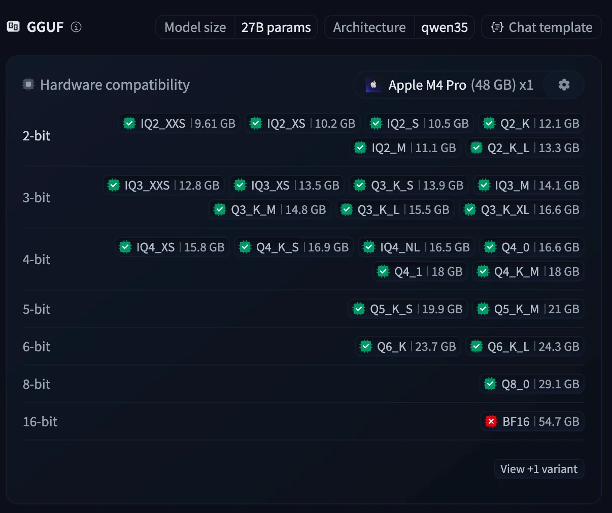
As you can see, I would not be able to fit Qwen3.5-27B at BF16, but thanks to quantization I am able to run such a model within my hardware capabilities.
What is inside a number?
To understand how quantization works, we first need to take a step back and look at how numbers are represented in computers.
You might remember Avogadro’s constant from chemistry class, defined as:
The sign tells us whether the value is positive or negative. The is the significand, which carries the significant digits, while the is the exponent, which determines the scale.
Binary floating-point uses the same basic idea, but represents the significand using binary digits (0s and 1s) and scales it using powers of 2. For example, a binary number might be written as , where is the significand and is the exponent.
The bits used to store the number are divided into a , an and a . The fraction stores the bits after the leading 1 of the significand. So for , the fraction stores 101. Since the significand is usually written in normalized form, the leading 1 is known in advance and does not need to be stored.
Ignoring some details of how the exponent is encoded (there’s a bit of bias trickery involved), we can think of the value as:
There are many different ways to store floating-point numbers in binary. FP32 and FP16 are defined by IEEE 754. BF16 follows the same broad design, while the FP8 and FP4 encodings below come from the Open Compute Project’s FP8 and Microscaling specifications.
More exponent bits allow us to represent a wider range of numbers, from very small to very large. More fraction bits provide greater precision, allowing us to represent numbers more accurately. Different formats divide their available bits between range and precision in different ways:
| Format | Sign | Exponent | Fraction | Notes |
|---|---|---|---|---|
| FP32 | 1 | 8 | 23 | wide range & high precision |
| FP16 | 1 | 5 | 10 | less range but more precision than BF16 |
| BF16 | 1 | 8 | 7 | FP32’s exponent range, lower precision |
| FP8 | 1 | 4 | 3 | You should get the gist by now+precision -range |
| FP8 E5M2 | 1 | 5 | 2 | more range, less precision |
| FP4 E2M1 | 1 | 2 | 1 | not much headroom here! |
Exponent bits buy range. Fraction bits buy precision.
FP16 (Half Precision) and BF16 (Brain Floating Point) make this trade-off quite clear. Both use 16 bits, but FP16 gives more bits to the fraction, while BF16 keeps the same eight-bit exponent as FP32. Avogadro’s number wasn’t chosen by accident! It is so large that the difference becomes easy to see:
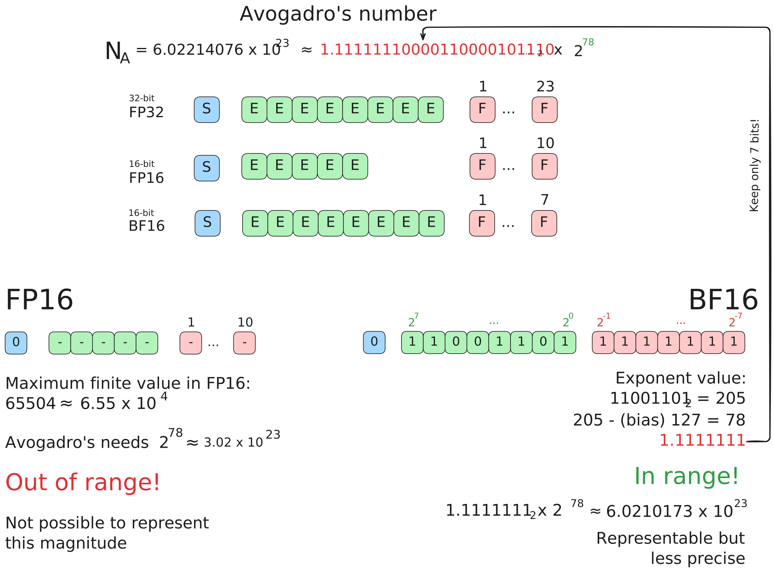
BF16 has enough range to represent Avogadro’s number, while FP16 does not. But for values that fit within both formats, FP16’s extra fraction bits let represent numbers more precisely.
Sixteen possible patterns
Once we get down to 4 bits, there are not many options left. Four bits can only represent different patterns (from 0000 to 1111). What those 16 patterns actually mean depends on the format. With INT4, they represent evenly spaced integers; with FP4, they represent values defined by a floating-point layout.
Probably easier to see than to explain:
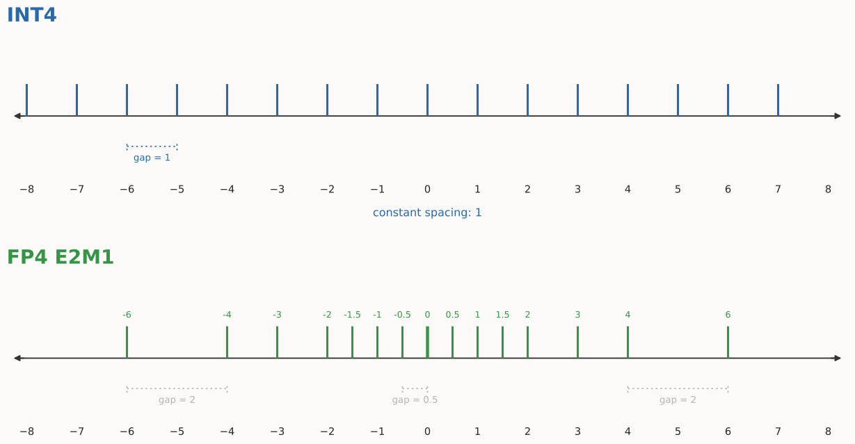
- INT4 uses a uniform grid (−8 to 7) with a constant step size of 1 across its representable range.
- FP4 E2M1 uses uneven spacing, keeping values close together near zero (0.5 apart) while taking larger jumps for bigger numbers (like 4 straight to 6).
The spacing between these points matters because it determines how closely values between them can be approximated. INT4 keeps the gap between neighboring values fixed at 1. FP4 uses smaller gaps near zero and larger gaps as the values grow. This lets it represent small values more closely while still reaching larger values with the same four bits. E2M1 also uses two patterns for and , so its 16 codes represent only 15 distinct values.
But what happens when the value we want to store falls between two of those representable points?
Rounding to a grid
In a neural network, the values we usually want to compress are its weights. If we start with some original value , quantization represents it as a small integer code , together with the metadata needed to interpret that code, which is usually shared by many weights at once. When we use the value again, the code and that metadata are used to reconstruct an approximation :
The difference between and is the quantization error.
An easy way to picture this is with a grayscale image. Below, the same image is represented using fewer and fewer intensity levels.
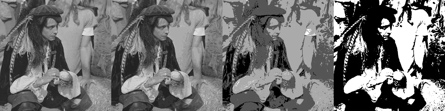
From left to right: 8-bit (256 levels), 4-bit (16 levels), 2-bit (4 levels) and 1-bit (2 levels) grayscale.
For model weights, we need to decide where those representable levels should sit. We keep a fixed set of integer codes, but use a scale to determine what one step between them is worth. So the first question is how wide the grid needs to be.
A simple symmetric quantizer starts by finding the largest absolute magnitude. We call it , then use the range from to . At 4 bits, the integer codes run from to and the scale is simply . To quantize a weight, we divide it by the scale and round it to the nearest code.
A signed 4-bit integer normally runs from to , but has no positive counterpart. This quantizer therefore uses the restricted range from to , deliberately leaving one code unused so that every negative level has a matching positive one. That is different from the FP4 example above: there, two patterns represent the same value, and ; here, one pattern is omitted. Some real formats use the full range instead, as we will see when we look inside llama.cpp’s formats.
The asymmetric version used here builds its grid from the smallest and largest weights, extending that interval to include zero when necessary. Since the range does not have to be centered, zero will not necessarily line up with code 0. A zero-point tells us which code should mean zero, so the grid can sit off-center rather than being forced to spread symmetrically around zero. This is one common affine quantizer, not a rule that every asymmetric format follows.
Symmetric
range −1.14 to 1.14
| weight x | −0.76 | −0.31 | 0.00 | 0.18 | 0.44 | 0.48 | 1.14 |
|---|---|---|---|---|---|---|---|
| code q | -5 | -2 | 0 | 1 | 3 | 3 | 7 |
| back x̂ | −0.81 | −0.33 | 0.00 | 0.16 | 0.49 | 0.49 | 1.14 |
Asymmetric
range −0.76 to 1.14
| weight x | −0.76 | −0.31 | 0.00 | 0.18 | 0.44 | 0.48 | 1.14 |
|---|---|---|---|---|---|---|---|
| code q | 0 | 4 | 6 | 7 | 9 | 10 | 15 |
| back x̂ | −0.76 | −0.25 | 0.00 | 0.13 | 0.38 | 0.51 | 1.14 |
0.44, 0.48 both become code 3 on the symmetric grid. The asymmetric grid keeps them apart as codes 9, 10.Values between grid points are rounded to the nearest point and values outside the range are clipped. When we convert the code back, we recover the chosen grid point rather than the original value.
We can put the same basic idea into a small NumPy function:
import numpy as np

def quantize(x, bits=4, symmetric=True):
    """Return the quantized codes, plus how to interpret them."""

    x = np.asarray(x)

    if symmetric:
        qmax = 2 ** (bits - 1) - 1  # 7 for 4-bit: codes run from -7 to +7
        scale = np.abs(x).max() / qmax
        scale = 1.0 if scale == 0 else scale

        q = np.clip(np.round(x / scale), -qmax, qmax)
        return q, scale, 0  # zero-point is fixed at code 0

    # Asymmetric: the grid does not have to be centered on zero.
    qmax = 2 ** bits - 1  # 15 for 4-bit: codes run from 0 to 15
    low = min(x.min(), 0)
    high = max(x.max(), 0)

    scale = (high - low) / qmax
    scale = 1.0 if scale == 0 else scale

    zero = int(np.clip(np.round(-low / scale), 0, qmax))

    q = np.clip(np.round(x / scale) + zero, 0, qmax)
    return q, scale, zero


def dequantize(q, scale, zero=0):
    """Reconstruct approximate floating-point values from the stored codes."""
    return (q - zero) * scale
That is why quantize hands back three things rather than one. The code alone does not tell us the value; we also need the scale and sometimes a zero-point, to interpret it.
The cost of rounding
Rounding a weight to the nearest grid point introduces an error. Sometimes that error is tiny and sometimes it is not. More importantly, the same amount of error does not necessarily have the same effect everywhere in the model.
A linear layer computes from its input activations . If quantization replaces with , the output changes by
A weight’s quantization error does not affect the model in isolation. What reaches the next layer is that error multiplied by the activation it meets, which means the same rounding error matters far more in a column fed by large activations than in a quiet one. That is why some weights can be rounded quite aggressively with little effect while errors elsewhere matter much more and we will come back to it when we look at why formats like Q4_K_M do not treat every tensor the same way.
A symmetric grid is often a good fit for weight distributions that are roughly centered around zero. But there is a catch! Remember how it gets built? It looks at the largest absolute value and uses that to set the scale. That means one unusually large weight can decide the spacing for all the others.
Say a thousand weights sit in and one is off at . Now , the scale is and the nearest non-zero grid points are all the way out at . Anything below roughly rounds to code 0, which in our case is nearly everything.
Symmetric
range −12.00 to 12.00
| weight x | −0.76 | −0.31 | 0.00 | 0.18 | 0.44 | 0.48 | 12.00 |
|---|---|---|---|---|---|---|---|
| code q | 0 | 0 | 0 | 0 | 0 | 0 | 7 |
| back x̂ | 0.00 | 0.00 | 0.00 | 0.00 | 0.00 | 0.00 | 12.00 |
Asymmetric
range −0.76 to 12.00
| weight x | −0.76 | −0.31 | 0.00 | 0.18 | 0.44 | 0.48 | 12.00 |
|---|---|---|---|---|---|---|---|
| code q | 0 | 1 | 1 | 1 | 2 | 2 | 15 |
| back x̂ | −0.85 | 0.00 | 0.00 | 0.00 | 0.85 | 0.85 | 11.91 |
12.00. Symmetric quantization sends every ordinary weight to code 0.On the symmetric grid, all six ordinary weights round to zero. The asymmetric grid does a little better here because the zero-point lets it shift the grid toward the weights, but five of the six still end up squeezed into just two codes. The underlying problem is not symmetry versus asymmetry: one scale has to work for everything.
This example is exaggerated to make the problem easy to see. Real weight distributions are not usually as extreme as this, and the especially large outliers associated with LLM quantization are often found in the activations, the numbers flowing between layers, which is one reason quantizing just the weights is easier. But weights still vary since one part of a weight matrix might contain mostly small values while another contains larger ones. If they all share one scale, the grid has to accommodate both, and some of its limited precision goes to waste.
We could clip the outlier and hope it was not important. Or we could stop asking every weight to share the same grid.
One scale becomes many
Instead of choosing one scale for an entire tensor, we can split the weights into smaller groups and give each group its own. Now an outlier only distorts the grid for the weights around it, rather than for everything else. The smaller those groups get, the more closely each grid can fit the values it actually has to represent.
But those extra scales are not free. Say we quantize a group of 32 weights at 4 bits each. The weights themselves take 16 bytes. Add a 2-byte FP16 scale and the whole group takes 18 bytes:
So our “4-bit” weights take 4.5 bits each: four for the code and half a bit of scale spread across the group. Smaller groups give us grids that fit their weights more closely, but they also mean storing more scales. Larger groups make that metadata cheaper, but then each scale has to cover more values, which starts bringing back the problem we were trying to solve.
This balance shows up everywhere in real quantization formats. The 4-bit code is only part of what gets stored. Scales, zero-points and other metadata take space too, so “4-bit” does not necessarily mean exactly 4 bits per weight.
MXFP4 and NVFP4 make this especially easy to see. Both use the same 4-bit E2M1 values we saw earlier, but they make different choices about the groups and scales around them.
MXFP4 groups 32 values together and stores an 8-bit E8M0 scale for each group. E8M0 uses all eight bits for the exponent, so its scales are restricted to powers of two:
NVFP4 uses smaller groups of 16 and an 8-bit E4M3 scale:
That extra quarter of a bit buys two things:
- a scale for every 16 values instead of every 32
- a scale format that can represent values between powers of two, not just the powers themselves
NVFP4 also adds a second FP32 scale shared across the whole tensor, though spread over that many weights its per-value cost is negligible.
llama.cpp’s GGUF quantization formats take another approach. Instead of storing a full-precision scale and offset for every small group, some of them quantize the metadata itself, which brings us to Q4_K_M.
Decoding Q4_K_M
Before we look at the struct definitions, the overall structure looks like this:
A model is a collection of tensors. A quantized tensor is an array of blocks and each block contains both the low-bit weight codes and the metadata needed to interpret them. As we go through the formats below, keep two questions in mind: how many weights go in a block and what metadata goes with them?
A simple example is Q8_0:
#define QK8_0 32
typedef struct {
    ggml_half d;         // shared FP16 scale factor for the 32 quantized values (2 bytes)
    int8_t    qs[QK8_0]; // 32 signed 8-bit quantized values (32 bytes)
} block_q8_0;            // total: 34 bytes
Each block represents 32 weights. Let be the original floating-point value of the -th weight and the integer code we store for it. To quantize it, llama.cpp finds the largest absolute value in the block and chooses
then stores each weight approximately as
Reading it back is just
So the code only becomes a weight once you apply its scale. If , the reconstructed value is and can be different for every block.
The reference implementation computes the scale in FP32 to choose the codes, then stores an FP16-rounded copy for dequantization.
That also means Q8_0 is not actually 8 bits per weight:
Q4_0 takes the same basic structure and cuts the codes in half. The block still represents 32 weights and still stores one FP16 scale, but each weight now gets a 4-bit code instead of an 8-bit integer. Two codes fit in each byte, so this is exactly the 18-byte block from earlier: 16 bytes of weight codes plus a 2-byte scale, or 4.5 bpw.
Unlike the restricted symmetric example above, Q4_0 uses the full range from to . If is the signed value with the largest magnitude, its working scale is , which maps exactly to code . Since the codes reach only in the other direction, the grid takes eight steps on the side is on and seven on the other and comes out negative whenever is positive.
Q4_1 adds an FP16 minimum , allowing the grid to shift instead of being tied to zero:
In the reference quantizer, is simply the block’s minimum, so the range does not have to include zero. That extra flexibility costs another two bytes of metadata. The block now takes 20 bytes:
or
Q4_0 and Q4_1 are older designs that llama.cpp still supports. Their simple block layouts make them useful examples, but the K-quants that came later use finer-grained metadata to get more quality out of the same bytes.
Q4_K is a good example. A block contains 256 weights, divided into eight groups of 32. Like Q4_1, each group gets its own scale and offset. But storing two FP16 values for every group would be expensive: eight groups would need 32 bytes of metadata before we had stored a single weight.
Q4_K compresses that metadata too. The eight scales and eight offsets are stored as 6-bit codes, taking just 12 bytes altogether. Two FP16 values, and , are then shared across the whole 256-weight block and used to interpret those codes.
So a Q4_K block has two levels of scaling: FP16 values shared by the whole block, and 6-bit scale and offset codes for each group of 32 weights. The weights themselves are still stored as 4-bit codes. The struct describes exactly this layout: 4 bytes of FP16 super-block metadata, 12 bytes of quantized scales/offsets, and 128 bytes of 4-bit weight codes.
If we call the 6-bit scale code for group , and its 6-bit offset code , then a reconstructed weight is:
Here is a 4-bit code from 0 to 15. The minus sign is important since represents the magnitude of a quantity subtracted from the scaled code, rather than a literal minimum added as in Q4_1. The Q4_K quantizer fits these values to reduce reconstruction error rather than simply storing each group’s exact minimum and maximum.
blockd 0.002506scale unitdmin 0.017502offset unit
x̂3,4=(0.002506×33)d s3×11q3,4−(0.017502×36)dmin m3=0.2797
The 4-bit weight codes take 128 bytes, so the whole block takes
or
So Q4_K gets back to the same 4.5 bpw as Q4_0, while still giving every 32 weights their own scale and offset. The trick is that the metadata used to interpret the quantized weights is itself quantized.
| Format | Weights/block | Metadata | Weight codes | Total | bpw |
|---|---|---|---|---|---|
Q8_0 | 32 | FP16 scale | 32 x 8 bits | 34 B | 8.5 |
Q4_0 | 32 | FP16 scale | 32 x 4 bits | 18 B | 4.5 |
Q4_1 | 32 | FP16 scale + FP16 minimum | 32 x 4 bits | 20 B | 5.0 |
Q4_K | 256 | 2 x FP16 + 16 x 6-bit codes | 256 x 4 bits | 144 B | 4.5 |
So that is Q4_K. But what about the _M in Q4_K_M? Well, Q4_K is a tensor type, while Q4_K_M is a model quantization recipe.
A tensor with type Q4_K uses the 256-weight blocks above. A model quantized as Q4_K_M, however, does not necessarily store every tensor that way. llama.cpp uses Q4_K as the main type for the recipe, while selected tensors can be stored at higher precision.
The _S and _M suffixes stand for Small and Medium. The exact mixture comes from hard-coded rules and depends on the model architecture, layer count, tensor shapes and conversion options and is not dynamically inferred from measured tensor sensitivity.
We can see this in practice with several versions of Qwen3.5-0.8B that I quantized using different recipes. I used a small model so it was easy to convert repeatedly and inspect and we’ll return to these same files later when we look at what quantization actually changed. For now, here are the tensor types each recipe produced:
Q8_0
  195 Q8_0
  140 F32

Q4_0
  194 Q4_0
  140 F32
    1 Q6_K

Q4_1
  194 Q4_1
  140 F32
    1 Q6_K

Q4_K_S
  187 Q4_K
  140 F32
    7 Q5_K
    1 Q6_K

Q4_K_M
  168 Q4_K
  140 F32
   27 Q6_K
Let’s look at Q4_K_S and Q4_K_M. Both have Q4_K in the name, but neither contains only Q4_K tensors. For this particular model and conversion, Q4_K_M has 27 tensors stored as Q6_K, compared with one Q6_K and seven Q5_K tensors in Q4_K_S.
One thing to keep in mind is that counting tensors does not tell us how much space they take up. The 140 F32 tensors, for example, are not necessarily a large fraction of the model’s parameters. Many are small tensors, while a single quantized weight matrix can contain millions of values. A complete Q4_K_M model therefore does not average exactly 4.5 bpw; its effective bpw depends on the mixture and the sizes of those tensors.
A final piece worth mentioning is the importance matrix (aka imatrix). I won’t dwell on it here, but llama.cpp’s imatrix tool records average squared input activations per input channel during representative model computations. An error in a matrix column fed by large activations can matter more than the same numerical error somewhere quieter, so the quantizer can give that error more weight when fitting scales, offsets and codes.
How do we know what changed?
So far we have looked at what quantization changes in the file: how the weights are represented, how blocks are laid out and how different tensors can end up at different precisions. Now we want to measure what that does to the model itself. Did it barely notice? Did it get worse? Did we quantize it into complete uselessness? There are many ways to measure this, but we will focus on a few common ones.
Perplexity
Perplexity measures how well the model predicts some text. If quantization makes the model worse at assigning probability to the tokens that actually occur, its perplexity goes up.
The model reads through a corpus token by token and at each position it assigns a probability to every token in its vocabulary; perplexity asks how much probability did it give to the token that actually appeared? A perplexity of 15 can be thought of roughly as the model being as uncertain as if it were choosing between 15 equally likely options.
In this experiment on WikiText-2, means perplexity rose by 4%. A ratio of would mean no change, while larger values indicate increasing degradation on this corpus.
BUT perplexity has a “weakness”. At each position, it only cares about the probability assigned to the token that actually appeared in the text. It does not care how the rest of the probability is distributed among all the other tokens. Two quantized models could therefore have very similar perplexity while their predictions still look quite different.
Kullback-Leibler divergence
This is where the KL divergence can be more helpful. Perplexity compares a model’s predictions with the text. KL divergence instead compares the quantized model directly with the original model. At each position, it looks at the entire probability distribution over the vocabulary and asks how far the quantized model has moved away from the original model :
When the KL divergence is near zero, the quantized model is distributing probability in roughly the same way. When it is larger, its predictions have moved further from the original model.
predicted next token for: “The cat sat on the ___”
Q4_K_Mp(mat) = 24%BF16 baseline: 30%
Perplexity tells us how quantization affected the model’s ability to predict the text, while KL divergence tells us how far its overall predictions moved from the original model. The two do not necessarily move together, although they often do. The probability of the observed token might barely change, while the probabilities of all the other tokens shift considerably. Perplexity would miss that change, while KL divergence would actually capture it.
Task benchmarks
At the end of the day, what really matters is whether the model can still do what you need it to do. Benchmarks like ARC-AGI and DeepSWE test this directly and instead of tracking shifts in token probabilities like perplexity or KL divergence do, task-based benchmarks simply ask: Can the model still actually solve the problem? We won’t be running full task benchmarks here, though. Instead, we’ll stick to comparing WikiText-2 perplexity and KL divergence against the original BF16 baseline.
So, what actually changed?
Now let’s see how our nine quantizations of Qwen3.5-0.8B compare. Q6_K and Q8_0 here are uniform (every quantizable tensor at that type), while the _M/_S suffixes elsewhere denote mixed recipes as with Q4_K vs Q4_K_M above:
perplexity above BF16KL divergence from BF16
BF161558 MBperplexity 15.4817the reference every row is scored against
Q4_1 is the only one that misses it.The line follows the best tradeoffs between size and quality, known as the Pareto front. For our experiment Q4_1 is the only format that falls outside it, because Q4_K_M is both smaller and better.
Let’s start with Q8_0. You will often see people online call it effectively lossless. While not exact, the numbers show why many providers serve models at this precision. It keeps the model almost intact while “halving” memory compared to BF16. Here it adds only 0.04% perplexity and keeps 98.9% of top-1 predictions.
Q4_0 and Q4_K_S show how different two 4-bit quantizations can be. Both use 4-bit codes and their files are almost the same size, 513 MB and 517 MB, yet Q4_K_S increases perplexity by only about 6%, compared with 21% for Q4_0. For roughly the same amount of space, one preserves the model much better than the other. This takes us back to the formats themselves, calling both of them “4-bit” hides quite a lot! Q4_K_S uses the per-group scales and quantized metadata we looked at earlier, while its quantization recipe can also keep some sensitive tensors at higher precision. The bit count is almost the same, but the way those bits are used is not.
Q4_K_S and Q4_1 give us a different kind of comparison because the two metrics do not quite agree on which one is better. Perplexity slightly favors Q4_1, while KL divergence favors Q4_K_S. The gap in perplexity is barely twice our margin of error, so the ranking might just be noise. With KL divergence, though, the gap is about seven times the error, pointing to a real difference. This makes sense: the two metrics track different things, so a small shift in one won’t necessarily show up the same way in the other.
As we move further left on the chart, the cost of compression becomes quite obvious. With Q2_K, perplexity is roughly six times higher than BF16 and the model chooses the same top token as BF16 only 44% of the time. At least for a model this small, we have pushed the compression too far. Larger models tend to handle the same quantization level better, which is one reason these more aggressive formats become more useful as models get bigger.
Of course, these exact numbers belong to this particular experiment. We tested one model, on one corpus, at one context length. A different architecture, a larger model, or an imatrix-aware quantization could shift the results. What matters here is the pattern we can already see in the chart. Fewer bits do not automatically mean a proportionally worse model and two formats with almost the same bit count can behave very differently.
So how much precision does intelligence actually need? In this case, less than we started with. The original model stores its weights in 16 bits, yet at around 4.5 bits per weight we can still keep more than 95% of its top-1 predictions unchanged.
Quantization is not just about using fewer bits. It is about using them wisely.
Want to reproduce the numbers yourself?
model:       Qwen/Qwen3.5-0.8B
llama.cpp:   b062ba735e5e15817f6a1dbdb84717ee3097f619
conversion:  --outtype bf16
context:     512
chunks:      32
corpus:      WikiText-2 raw test
quants:      Q8_0 Q6_K Q5_K_M Q4_K_M Q4_K_S Q4_1 Q4_0 Q3_K_M Q2_K
uv run python convert_hf_to_gguf.py \
./Qwen3.5-0.8B \
--outfile Qwen3.5-0.8B-BF16.gguf \
--outtype bf16
for q in Q8_0 Q6_K Q5_K_M Q4_K_M Q4_K_S Q4_1 Q4_0 Q3_K_M Q2_K; do
llama-quantize \
Qwen3.5-0.8B-BF16.gguf \
"Qwen3.5-0.8B-${q}.gguf" \
"$q"
done
# reference logits from the unquantized model
llama-perplexity \
-m Qwen3.5-0.8B-BF16.gguf \
-f wikitext-2-raw/wiki.test.raw \
-c 512 \
--chunks 32 \
--kl-divergence-base qwen3.5-bf16.kld
# perplexity and KL divergence together, per format
for q in Q8_0 Q6_K Q5_K_M Q4_K_M Q4_K_S Q4_1 Q4_0 Q3_K_M Q2_K; do
llama-perplexity \
-m "Qwen3.5-0.8B-${q}.gguf" \
-f wikitext-2-raw/wiki.test.raw \
-c 512 \
--chunks 32 \
--kl-divergence-base qwen3.5-bf16.kld \
--kl-divergence \
| tee "perplexity-${q}.log"
doneThe tensor-type tallies further up came from gguf_dump.py:
uv run python gguf-py/gguf/scripts/gguf_dump.py Qwen3.5-0.8B-Q4_K_M.gguf \
  | awk '/\| (Q[0-9A-Z_]+|F32|F16|BF16) +\|/ {print $(NF-2)}' \
  | sort | uniq -c | sort -nr
llama.cpp documents what these numbers mean in tools/perplexity.